Charlotte Gurr
After reading this article, you should be able to:
- Describe the purpose of correlation and regression analyses, including commonly used correlation tests and their interpretation;
- Describe and discuss the purpose of survival analyses, including how they are usually reported and analysed in a study;
- Describe the purpose of conducting a Cox proportional hazards model and the types of data provided.
This article is part of a comprehensive series exploring how to evaluate clinical studies when addressing information needs using a five-step process:
- Identifying study type or design;
- Appraising the journal, authors and study purpose;
- Critiquing the methods used;
- Analysing study data and results, and the discussion section;
- Understanding basic statistical tests.
This article explores the fifth step: understanding basic statistical tests. It is recommended that you read it in conjunction with the article ‘Understanding commonly used statistical tests’.
The statistical tests reviewed in the previous article in this series are used to determine the likelihood that any group differences found in the outcome measures resulted from the treatments. These tests involved analysing the effects of an independent variable (e.g. treatment used) that does not change in value during the study on the dependent variables (i.e. outcome measures) that change in value.
However, suppose both variables change in value during the study, and investigators wish to determine how changes in the values of one variable might affect the values of the other variable. Analyses of variables that both change in value are used to answer the following questions:
- Are there associations among the variables measured in the study groups?
- What predictions can be made for the population based upon the results obtained from the study sample?
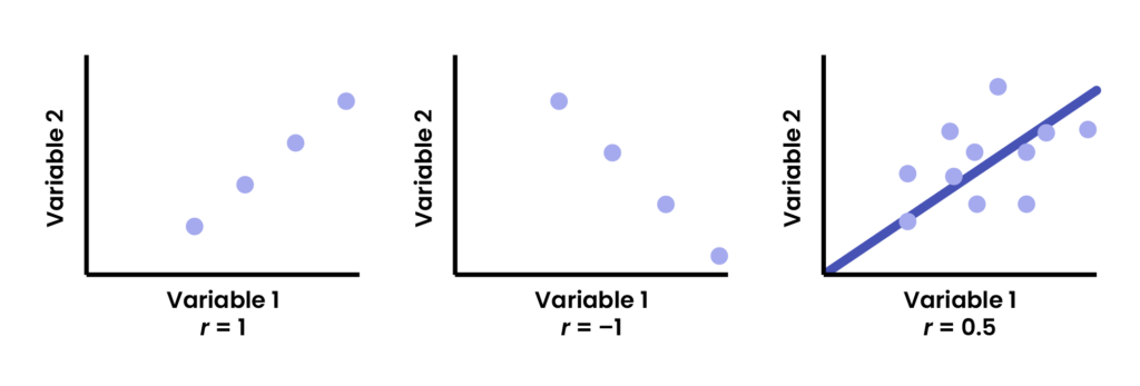
The association between two variables, both of which change in value, is called a correlation. There are not defined independent and dependent variables in a correlation. A correlation simply examines the relationship between two variables, or how the values of both change together without assuming any causal relationship. For example, suppose investigators decide to study the association between diazepam blood concentrations and a subject’s reaction time while driving. A correlation coefficient — represented as r — is used to quantify the strength and direction of a linear association (i.e. correlation) between two such variables. The values of r can range in value from −1 to 1 (see Figure 1):
- 0 indicates no linear association between the variables (i.e. whether the value of one variable increases or decreases has no effect on the value of the other variable);
- 1 (positive or negative) indicates perfect correlation, meaning as one variable changes in value the other variable changes by the same proportion;
- A negative r indicates a negative (i.e. inverse) association, meaning as one variable increases in value, the other variable decreases (or the reverse);
- A positive r indicates a positive association; as one variable increases (or decreases) in value, the other also increases (or decreases) in value;
- The closer the r is to 1 (in either direction), the stronger the correlation.
Figure 1: Illustration of correlation (r) values
Two common statistical methods are used to calculate a correlation coefficient r value: the Pearson r (or Pearson product-moment r) and the Spearman rank-order (rho) r. The Pearson r is parametric, meaning that the values for both variables should be continuous-level and normally (or near normally) distributed. The Spearman rank-order r is its nonparametric counterpart and is used when one or both variables are either ordinal-level, or continuous-level but not normally distributed.
Key point
A negative r can indicate a correlation as strong as, or stronger than, a positive r — it’s just that the direction changes. The following values for r provide a rough estimate of the strength of the correlation:
- Strong: −0.5 to −1 (or 0.5 to 1);
- Moderate: −0.3 to −0.5 (or 0.3 to 0.5);
- Weak: −0.1 to −0.3 (or 0.1 to 0.3);
- None: <−0.1 (or <0.1).
Worked example 1
In the previous diazepam example, the investigators report a correlation coefficient of r = 0.65 for diazepam concentrations and reaction time (in seconds) at a driving simulator.
How should this correlation be interpreted?
The positive value means that, as the diazepam concentration increases, reaction time increases as well. The value of 0.65 indicates a fairly strong correlation since the closer it is to 1, the stronger the correlation.
Key points
Keep in mind the following about the correlation coefficient r:
- r values are not directly proportional to each other — for example, r = 0.8 for one correlation analysis is not twice as strong as another r = 0.4;
- r values are on a continuum, with no precise cut-off for which correlation is ‘strong’ and which is ‘moderate’;
- The statistical significance of an r value can be calculated. Large sample sizes might find that an r value is ‘statistically significant’, meaning not likely a result of random or chance variability but owing to a real association between variables. However, the r might still represent a weak correlation;
- r2 (also called the coefficient of determination) is helpful for interpreting the degree of association between two variables. It represents the amount/proportion of variation in one variable that can be explained by the presence of the other variable. In the diazepam example, r2 = 0.652 = 0.42. This means that 42% of the variation in reaction time can be explained by knowing the diazepam concentration. The remaining 58% of reaction time variability would be due to other factors unrelated to diazepam concentrations;
- Just because there is a strong correlation between two variables does not mean that one variable caused the other. For example, a strong correlation might be found between walking one’s dog and the extent to which healthy foods are eaten. This does not mean that walking a dog causes a person to eat healthier foods (or that eating healthier foods causes one to walk a dog). They may be correlated because persons who exercise to a greater extent take better care of their overall health, including healthier eating habits.
Regression
Correlation only looks at the strength of an association between two variables. Suppose investigators want to predict what the value of an outcome will be in the presence of other variables and to explore the relationships among variables. Regression is used to explain the association among variables and an outcome and, importantly, provides a mathematical equation that can be used to predict an outcome measure’s value based upon the value of an independent (i.e. explanatory) variable. Four commonly used regression analyses are reviewed here:
- Simple linear regression (i.e. one continuous level independent variable; one continuous level outcome measure);
- Multiple linear regression (i.e. two or more categorical [nominal level] or continuous independent variables; one continuous level outcome measure);
- Simple logistic regression (i.e. one categorical or continuous independent variable; one categorical outcome measure);
- Multiple logistic regression (i.e. two or more categorical or continuous independent variables; one categorical outcome measure).
Note that the type of regression depends on whether the dependent variable is continuous level (i.e. linear regression) or categorical/nominal level (i.e. logistic regression). The number of independent variables determines whether the regression is simple (i.e. one independent variable) or multiple (i.e. two or more independent variables). An example of a multiple logistic regression analysis involves studying the relationship among age, gender, number of drugs taken, number of prescriptions received (i.e. a variety of categorical and continuous independent variables) and whether a person was more likely to die from prescription drug use (i.e. one categorical outcome — alive or dead).
A regression analysis provides estimated regression coefficients to describe relationships between the independent variables included and the outcome. In linear regression, the coefficients are generally reported directly. In logistic regression they are commonly converted to odds ratios, and in Cox regression models, they are commonly converted to hazard ratios (see Cox regression discussion below).
In linear regression, a regression coefficient represents the change in the outcome associated with a defined change in an independent variable, while considering the other variables in the analysis. For example, suppose a multiple linear regression analysis examined how every increase in Age of 5 years affected sleep time in minutes. Suppose the regression analysis also included several other independent variables. They reported a regression coefficient of +5.6 minutes for Age (per 5-year increase). This would be interpreted as, each 5-year increase in age was associated with an average of 5.6 extra minutes of sleep, while considering the other variables in that model.
Worked example 2
1. Investigators compared the efficacy of a new topical antibiotic to placebo to treat skin impetigo. The severity of the impetigo was scored after therapy using a Skin Infection Rating Scale (SIRS, range of scores = 0 – 15). The primary efficacy measure was ‘clinical success’, defined as a score of 2 or less on the SIRS. The investigators also wanted to determine whether the number of affected areas, the size of the areas and patient age could predict clinical success.
Which regression analysis should be used here?
a. Simple linear regression; b. Multiple linear regression; c. Simple logistic regression; d. Multiple logistic regression
Answer: Multiple logistic regression. There are several independent variables that are continuous (e.g. number of affected areas, size of area, patient age) and one categorical outcome measure (i.e. clinical success — patients would have a score of 2 or less, or not).
2. Investigators would like to determine if the measured abdominal (i.e. waist) diameter can be used to predict the body mass index (BMI).
Which regression analysis should be used here?
a. Simple linear regression; b. Multiple linear regression; c. Simple logistic regression; d. Multiple logistic regression
Answer: Simple linear regression. There is one continuous level independent variable (i.e. waist diameter) and one continuous level dependent variable (BMI).
Survival analysis
Clinical studies are often interested in determining whether a therapy makes a difference in the time until a certain outcome happens, such as a relapse or remission. Survival analysis is a collection of statistical methods used to analyse and compare data in which the outcome is the time until a specific event of interest occurs. Survival analysis is used by investigators to estimate treatment differences in the proportion of subjects who ‘survive’ (i.e. survival event) a given amount of time under the conditions of the study. This analysis examines the time between when subjects enter the study and when the subsequent event (i.e. outcome, dependent variable) occurs. The time to event (i.e. ‘survival time’) can be measured in any time unit (e.g. days, weeks, years).
When first developed, survival analysis focused on time to death (thus, the term ‘survival’). It is now used to examine time to other types of outcomes. Common survival events in clinical trials include death; development of a disease, medical condition, injury, or complication; failure or relapse; and recovery. Some examples in which survival analysis is used include:
- Time to relapse in cancer patients receiving drug therapy;
- Time to development of myocardial infarction or stroke in high-risk patients;
- Time to rejection or death in patients who receive a transplant.
Survival analysis methods
Estimating survival/event time is not as straightforward as it might appear for several reasons: patients enter a study at different times, the risk of an event might vary over time, and not all patients will have the event before the study ends. For example, if comparing time to relapse, some patients might not relapse before the end of the study, so the actual relapse (‘survival’) time is unknown. When the observations for patients stop before the event occurred, the times for such patients are referred to as censored, and these data need to be handled differently during the analyses. Why? If the event times for censored data are simply recorded using the time the study ended, the ‘survival’ could be underestimated since one does not know how many additional months or years the patients might have gone before experiencing the event.
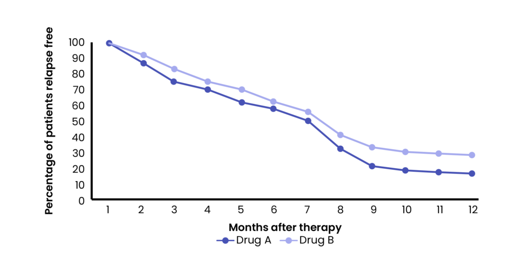
A commonly used method for determining the probability of ‘survival’ (i.e. time to event) is the Kaplan-Meier method. This method estimates and graphs, usually as a curve, the survival probabilities as a function of time. Survival curves from different treatments are generally placed on the same graph (see Figure 2).
Although Kaplan-Meier survival plots might seem to differ by appearance on a graph, the Kaplan-Meier method does not analyse whether the curves are truly significantly different from each other (i.e. whether any differences seen represented real treatment effects). Another statistical test, such as the log-rank test, is needed to check for statistical significance. The log-rank test is a popular statistical method used to test for differences in the Kaplan-Meier survival graphs/plots between groups (e.g. Drug A and Drug B in Figure 2) that takes the entire follow-up period into account. It tests the null hypothesis that there is no difference between groups in the probability of an event (e.g. death, adverse effect, etc.) occurring at any time point, by essentially comparing the observed events at each point with the number expected if the survival/event experience was the same in both groups. The log-rank test generates a p value to determine statistical significance. This test is most likely to detect a significant difference between groups when the risk of an event occurring is consistently greater for one group than another over time.
Figure 2: Example — Kaplan Meier curves
While Kaplan-Meier curves and the log-rank test indicate whether there are survival differences between treatment groups, the time to an event is often influenced by a variety of factors or variables (e.g. age, sex, underlying conditions, duration of illness, time in hospital, etc.) that a survival function alone cannot take into account. To explore the contributions of a variety of independent variables on survival estimates, a specific regression method known as the Cox proportional hazards model or Cox proportional hazards regression model is often used. Thus, think of the Cox Proportional Hazards model as a regression analysis for survival data.
This model is based on a hazard function, which simply means the risk or probability that an individual dies or experiences the event at a specific point in time, assuming they survived up to that point. With the Cox regression model, the dependent variable is the hazard/event risk (i.e. outcome) and the independent variables are the factors that the investigators feel might affect that outcome. The Cox model can estimate a treatment effect on the outcome after accounting for and separating out the effects of the other potentially contributing variables.
The Cox proportional hazards model also calculates hazard ratios and confidence intervals (CIs) for the independent variables involved in the model. The hazard ratio, abbreviated HR, calculates the risk of an event occurring in the treatment group compared with that in the control group taking into account differences in time. (Note: while this ratio is similar to relative risk [RR], the RR does not account for time). It is important to factor in the effects of time in a survival analysis since benefits or risks might vary based on time in the study — for example, a treatment might have greater benefit early during therapy and less efficacy later, while the control therapy might show more benefit later and less benefit earlier. The therapy benefits might also steadily increase, decrease or remain the same over time.
The HR in a survival analysis is defined as the ratio of the hazard or risk of the event occurring in the treatment group to the hazard or risk of the event occurring in the control/comparison group (assuming patients survived until that point). A HR = 1 indicates no difference between groups in the hazard or risk of the event occurring. With HR > 1, there was greater hazard or risk in the treatment group. For example, a HR = 2 means that a patient in the treatment group who has not experienced an event at a certain time has twice the chance of experiencing it by the next point in time compared to the control/comparison patients. A HR < 1 indicates less hazard or risk in the treatment group. For example, a HR = 0.5 means that a patient in the treatment group who has not experienced an event at a certain time has 50% of (or half) the chance of experiencing it by the next point in time compared to control/comparison patients.
Key points
Example — Cox proportional hazards regression model use in a study
COVID-19 was associated with high mortality early in the pandemic, particularly in areas of Europe at the centre of the first outbreak (e.g. the Lombardy region in Italy). Since the importance of identifying factors that might significantly impact the risk of death was clear, a retrospective study was conducted to examine the effects of several risk factors on time to death in critically ill patients with confirmed COVID-19 admitted to the intensive care unit (ICU) in Italy.
The outcome measure was time to death in days from ICU admission, and several independent variables/factors possibly associated with patient mortality were examined using Cox models, including: age; male sex; respiratory support; presence of hypertension, hypercholesterolemia, heart disease, Type 2 diabetes, malignancy, or Chronic obstructive pulmonary disease (COPD); taking an angiotensin-converting enzyme inhibitor, Angiotensin-II receptor blockers, statin, or diuretic; and positive end-expiratory pressure (PEEP) and fraction of inspired oxygen at admission.
The Cox models reported HRs with CIs. Those factors found to be significantly associated with greater mortality (HRs > 1 overall and with CIs) included: age, male sex, hypercholesterolemia, diabetes, COPD history, and decreased PEEP and fraction of inspired oxygen at admission. Although having the limitation of being retrospective, this study used Cox proportional hazards models to identify several variables that could be important risk factors for greater mortality in severely ill COVID-19 patients.
Grasselli G,et al. Risk factors associated with mortality among patients with COVID-19 in intensive care units in Lombardy, Italy. JAMA Intern Med. 2020 Oct 1;180(10):1345-1355. doi: 10.1001/jamainternmed.2020.3539
A summary of key points and how to apply the information from this article to practice follow.
Key points
- A correlation coefficient (r) provides the extent of linear association between two variables; it can only assume a value from −1 to 1 and a negative value indicates an inverse association between variables;
- Regression goes beyond a correlation in that it provides a mathematical equation to predict an outcome measure’s value based on the values of the independent variables studied;
- Survival analysis provides excellent tools for examining the time to an event occurrence;
- A hazard ratio (HR) is used in survival analysis to provide the hazard or risk of an event occurring in the treatment group compared to the control; it differs from relative risk (RR).
How to apply to practice
When evaluating the correlation, regression and survival analyses used in a clinical study, consider the following:
- Look at the actual value of r calculated for a correlation coefficient, regardless of whether it was found to be statistically significant. Weak r values, indicating a lack of meaningful association between variables, could be statistically significant if the study enrolled a large sample size;
- r2 can provide a good way to interpret correlation coefficients by estimating the proportion of variability in one variable that can be explained by the other;
- Look for the results from statistical analysis (e.g. log-rank test) to determine whether Kaplan-Meier curves differ significantly from each other;
- While a HR is similar to that of a RR, the HR takes time to event into account in its use and interpretation.
Summary
This article provided an overview of correlation, used to determine relationships between variables in a study, regression, used to examine the relationships between an outcome and one or more factors that might influence that outcome, and survival analyses, methods used to analyse and compare data in which the outcome is time until a specific event of interest occurs. Each of these types of analyses provides clinicians with valuable information by examining specific relationships among the study data.
Self-assessment questions
A study examines the association between quality of life in arthritis, measured using a scale of from 3 (excellent) to 0 (poor), and the extent of joint erosion (measured in millimeters). The study reports an r = −0.57 (Spearman rank r) for this association. Answer questions 1-4 about the r value reported.
QUESTION 1
What does the negative value of r indicate?
QUESTION 2
Was it appropriate to use the Spearman rank r to determine the correlation?
QUESTION 3
Is the correlation reported considered to be strong?
QUESTION 4
How much of the variability in the patients’ quality of life scores can be explained by variations in the extent of joint erosion?
QUESTION 5
Many patients fail to respond to treatment with anti-tuberculosis drugs. A study was performed to predict the effect of sex, age, weight and yearly income on the likelihood of success or failure with tuberculosis therapy. What type of regression analysis would be represented here?
A: Simple linear regression
B: Multiple linear regression
C: Simple logistic regression
D: Multiple logistic regression
QUESTION 6
Investigators studied whether certain characteristics were associated with systolic blood pressure (SBP) in 320 adults with hypertension. They performed a multiple linear regression analysis, with SBP (mm Hg) the dependent variable. Age, body mass index (BMI), and daily sodium intake were included as independent variables.
Results:
| Independent variable | Regression coefficient | 95% CI | P value |
| Age (per 10 years) | +3.2 mm Hg | +1.5 to + 4.9 | <0.001 |
| BMI (per 1 kg/m2) | +0.8 mm Hg | +0.1 to +1.3 | 0.002 |
| Sodium intake (per 1,000 mg/day) | +2.5 mm Hg | +0.7 to +4.3 | 0.007 |
How should these findings be interpreted?
QUESTION 7
Kaplan-Meier curves show whether two therapies are statistically significantly different from one another in producing changes in the time to an event occurring. True or false?
A: True
B: False
QUESTION 8
The HR is considered the same as other measures of risk such as relative risk since it shows the hazard or risk of an event occurring at the end of a study period. True or false?
A: True
B: False
Answer guidance
QUESTION 1
There is an inverse linear association between quality-of-life ratings and extent of joint erosion, or, as the extent of joint erosion increases, the quality-of-life ratings decrease.
QUESTION 2
Yes: The Spearman rank r is used to determine the linear correlation between two variables when one or both are either ordinal-level or continuous-level but not normally distributed. The quality-of-life rating is ordinal-level (ranked data) and joint erosion measured in millimetres is continuous level, which might or might not be normally distributed. Normal distribution is not a concern in this specific example since the ordinal-level data would preclude use of the Pearson r correlation, which required both variables to be continuous and normally distributed.
QUESTION 3
It is considered to be moderate to strong since it is in the range of 0.5–1, but close to the lower end of 0.5.
QUESTION 4
The value of r2, the coefficient of determination, represents the amount/proportion of variation in one variable that can be explained by changes in the other variable. In this example, r2 = 0.325, which means that 32.5% of the variability in the arthritis quality of life ratings can be explained by the presence of the joint erosion. This indicates that other unexplained factors are responsible for most (67.5%) of the variability in the quality-of-life ratings.
QUESTION 5
D: Multiple logistic regression – a nominal dependent variable (likelihood of success or failure with tuberculosis therapy) is involved, with several (more than one) independent variables that include continuous and nominal level variables.
QUESTION 6
With this multiple regression example, after accounting for the other variables included in this model, each 10-year increase in age was associated with an average 3.2-mm Hg higher SBP. Similarly, each 1-kg/m² increase in BMI was associated with a 0.8-mm Hg higher SBP, and each additional 1,000 mg of daily sodium intake was associated with a 2.5-mm Hg higher SBP. All three associations were statistically significant.
QUESTION 7
False: Kaplan-Meier curves graphically illustrate the proportion ‘surviving’ or experiencing an event over time, but themselves do not provide whether any differences seen are statistically significantly different. A statistical test, commonly the log-rant test, is used to show statistical significance.
QUESTION 8
False: The hazard ratio (HR) provides the ratio of the hazard/risk of an event occurring in the treatment group compared to the hazard/risk of the event occurring in the control/comparison group, taking time into account. It differs from a measure such as relative risk that is typically done one time at the end of a treatment period. For example, a HR = 1.3 indicates that there was a greater hazard/risk of an event occurring in the treatment group; and, a patient in the treatment group who has not experienced the event at a certain time has 1.3x the chance of experiencing the event by the next point in time compared to the control/comparison patients.
Acknowledgements
This article was adapted from Drug Information and Literature Evaluation, Second Edition, previously published by Pharmaceutical Press.
A full list of resources and materials used to prepare the book can be accessed from the bibliography page.